Accelerated Kernel Density Estimation in CUDA

Our S-KDE implementation operates on 3D datasets and consists of four phases. First, on the CPU, we evaluate the dataset and construct a covariance matrix, which is inverted to produce an ellipsoid kernel matrix. The memory is then transferred to the GPU.

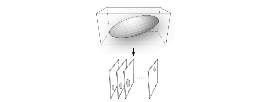
In the next phase, each kernel in parallel is chopped into slices along the Z-axis (parallel to the XY plane). This process produces a list of "slice ranges", where a slice range is simply the Z-axis range of each kernel, snapped to the evaluation space cell grid.

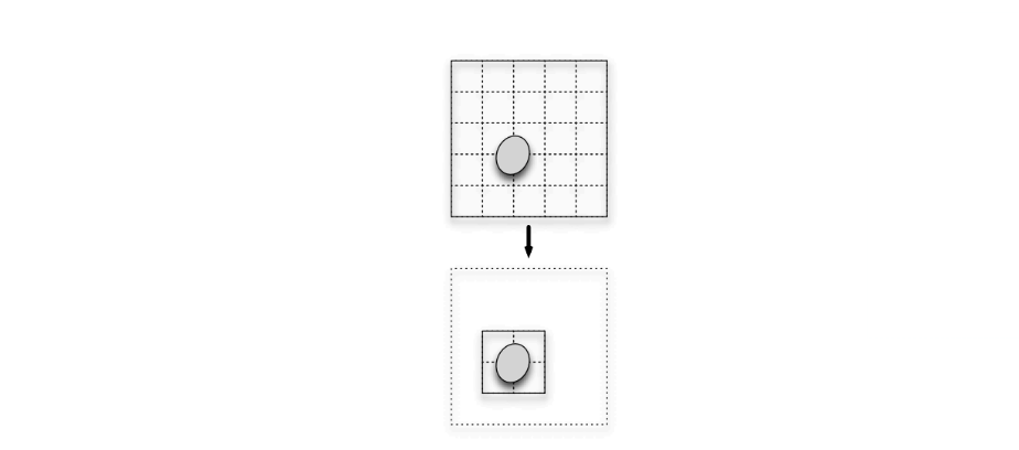
In the third phase, each slice of each kernel is cropped in parallel to the AABB of the kernel cross section in that slice, which is elliptic. The result of this phase is a list of "grid ranges", each of which indicates the X and Y range of cells that must be evaluated for the kernel slice at a given Z.

In the final phase, each cell of each slice of each kernel is evaluated in parallel and accumulated using an atomic operation.

We have evaluated our S-KDE implementation against a naive CPU-based evaluation-space implementation, a naive GPU-based sample-wise implementation (without Chop and Crop), and finally the authors' CPU-side OpenMP implementation of the full S-KDE algorithm.

For each evaluation run, we first generated five gaussian distributions, with centers and variances sampled uniformly between -1 and 1 in XYZ, and used these distributions to generate N samples. We defined an evaluation space between -5 and 5 in XYZ, divided into M³ grid cells. The bandwidth was fixed at 1 and we used an Epanechnikov kernel defined by the inverse of the covariance matrix of the dataset.

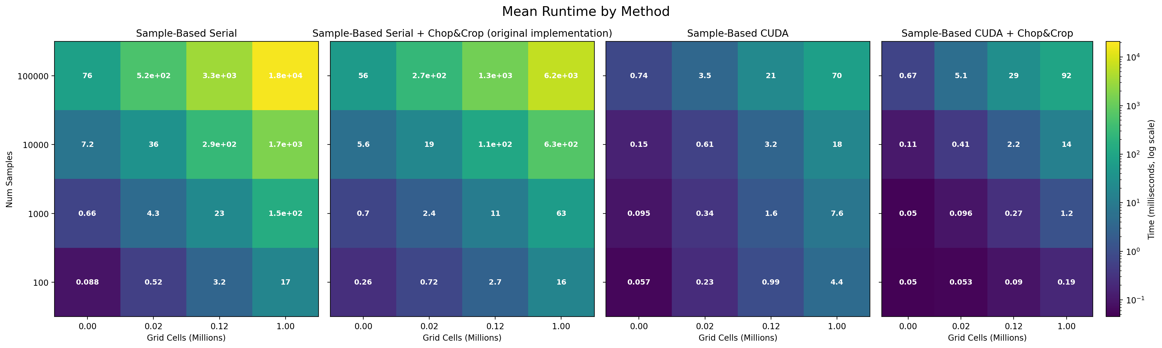
We tested sample counts (N) of 100, 1000, 10000, and 100000, and grid resolutions (M³) of 10³, 25³, 50³, and 100³. There were three repetitions per experimental condition, and for CUDA implementations we additionally ran three warmup calculations, whose timiings were discarded.

The tests were run on Windows Subsystem for Linux on an Intel Core Ultra 9 185H with 16GB RAM, and an Nvidia RTX 4070 8GB (Laptop), with CUDA 12.6.1.

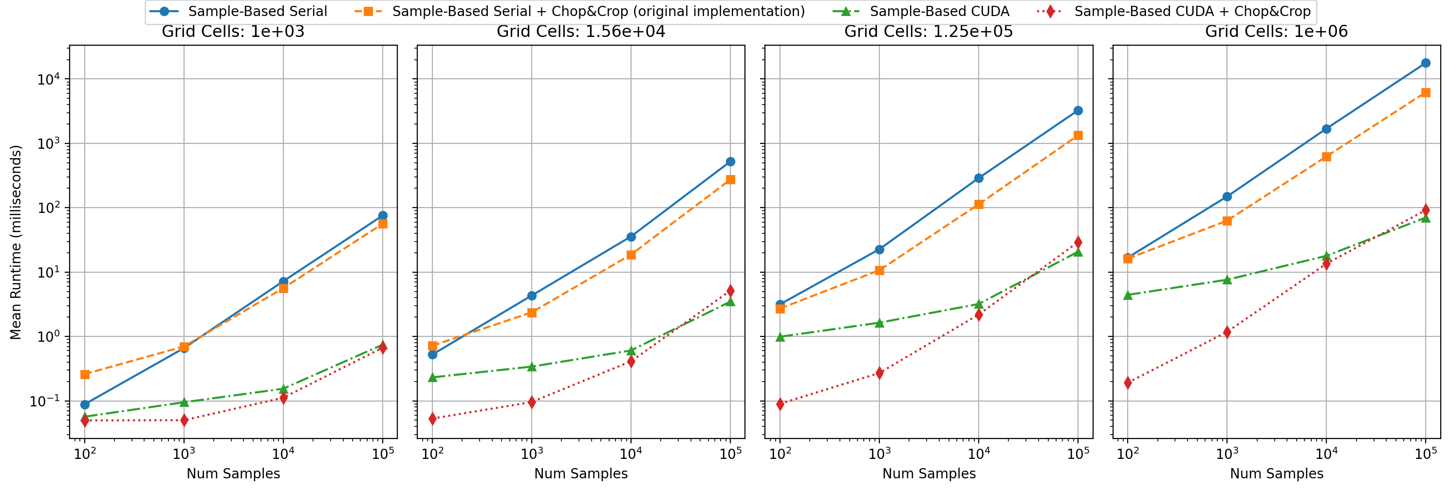
First, we can clearly observe that with the number of samples and the number of evaluation points, the runtime gets larger. This is true across all methods. Notably, the CUDA implementations are an order of magnitude faster than serial ones.

We can clearly see that the sample-wise parallelism results in much better scaling than serial approaches.

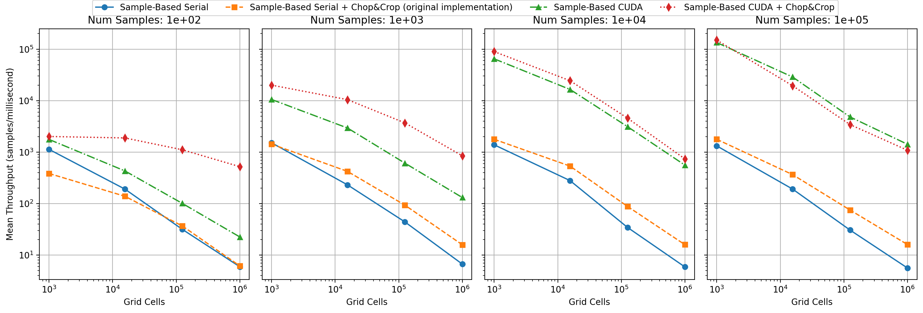
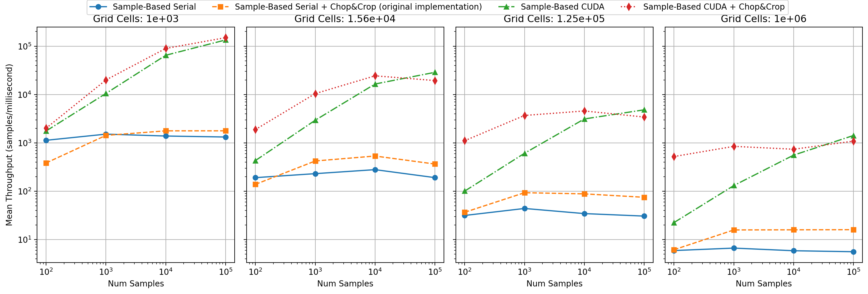
If we inspect the throughput of our algorithms under different conditions, we can see some clear trends, such as higher throughput achieved by CUDA implementations in large-dataset scenarios. Expectedly, all the algorithms behave worse as the total number of evaluation cells increases.

We suspect that the biggest bottleneck in the parallel algorithms are: (1) stall incurred during atomic operations when accumulating the PDF, (2) non-coallesced access patterns. In the future, both of these potential improvements could be investigated.

For more benchmarking plots and profiling analysis, we reference the relevant slides.

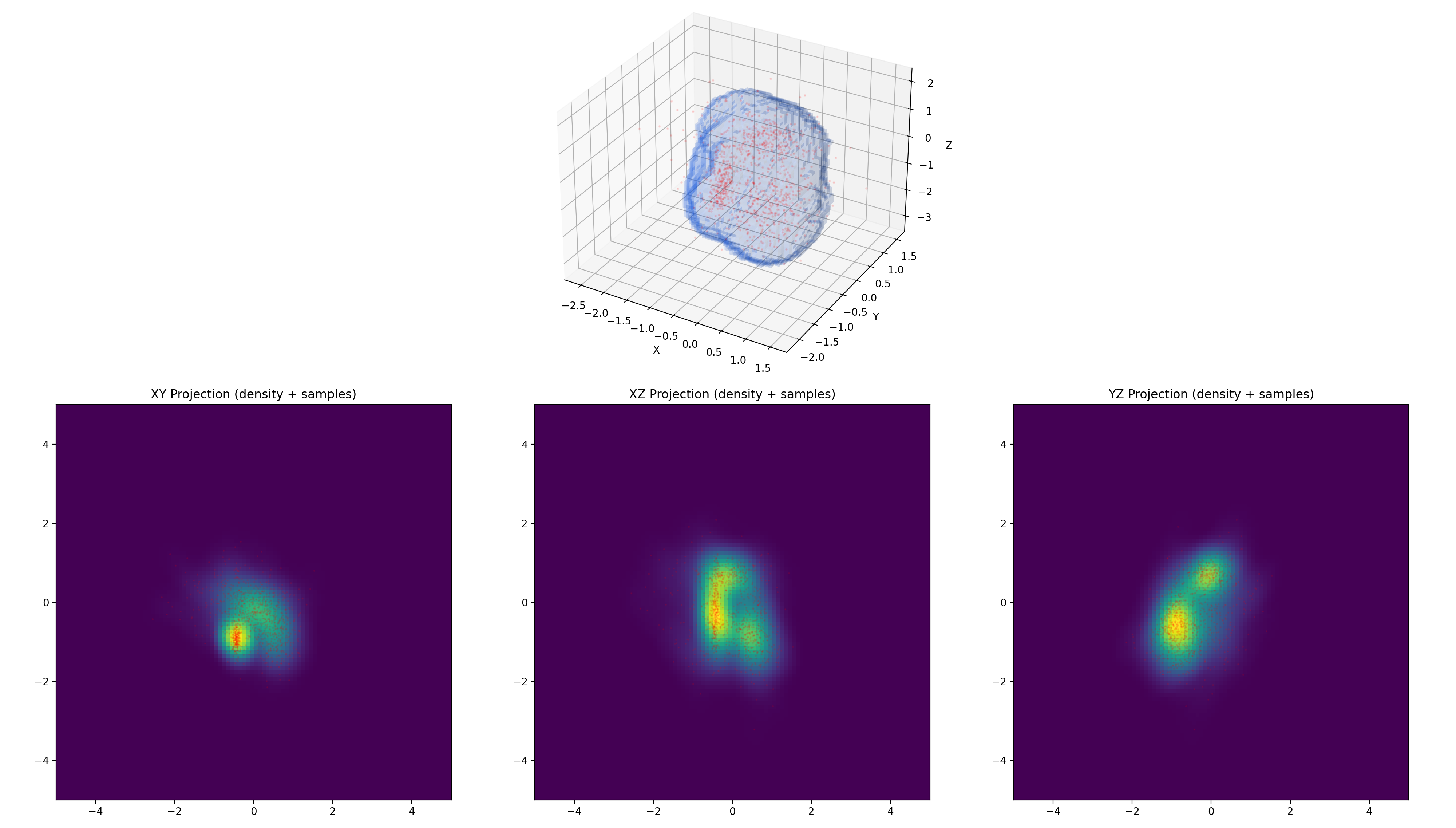
We have also built a small OpenGL application to visualize the results of the S-KDE algorithm. Because our implementation runs entirely on the GPU, we can take advantage of CUDA's OpenGL interoperability to visualize the results directly, without ever passing the data to the CPU.

On the right hand side of the window, the application visualizes the final PDF using raymarching and a simple linear transfer function. On the left hand side, it visualizes the slices from the chop and crop steps of the S-KDE algorithm. Areas inside the ellipsoid kernel are shown in yellow, appearing on the slices as 2D elliptic cross sections. In green are shown the cropped bounds of the slice, that is, the cells that are actually evaluated. The full bounds of the slice are shown in gray, and can be toggled on or off.